DPKAI Aqualab is a desktop research tool for aquaculture scientists, farm managers, and water
quality analysts. It connects a standard USB microscope or video file to a suite of trained
detection detection engines and delivers real-time organism counts, density measurements, trend dashboards,
and structured database records — all in one window.
🦠
Multi-Mode Detection
Switch instantly between Algae (27 + species), Total Algae Count, WBC subtypes, Bacteria, and Live Feed modes using the same camera or video file.
🆔
Persistent ID Tracking
Each cell receives a stable track ID across frames. A session-long "counted gallery" prevents the same organism from being counted twice even after brief disappearance.
📐
Calibrated Density
Calibrate with a scale bar, draw a ROI, and get live cells /mm² and /m² density that is saved alongside every detection record.
📊
Interactive Dashboard
Seven chart types (scatter, bar, pie, line, histogram, box-plot, table) auto-refresh after every save. Export any chart to a PNG file.
🗄️
SQLite + Excel
All detections stored locally in a SQLite database. Yearly Excel workbooks are regenerated automatically after every save.
🔒
Secure Data Management
Password-protected access for editing, deleting, and querying raw records via a built-in SQL browser. Supports sign-up, login, and token-based password reset.
DPKAI Aqualab v0.1 — video display left, detection controls right.
2
Quick Start
From first launch to your first saved detection in under five minutes
1
Place detection engine files next to the script
Copy algae.pt, wbc.pt, bacteria.pt, and total_algae.pt into the same folder as dpkai_aqualab_v0.1.py. Also place custom_botsort.yaml there if you want custom tracking parameters. The app loads WBC mode automatically at startup.
2
Enter your username and site information
Type a name in the Username field and click Save. Then select or create a Site Name and Tank/Pond/Treatment. These are recorded with every detection for traceability.
3
Choose a detection mode
Click one of the tabs in the Detection Mode panel — Algae, Total Algae, WBC, Bacteria, or Live Feed. The corresponding .pt detection engine loads automatically.
4
Load an image, video, or camera
Click 📸 Process Image for a still image, 🎬 Process Video for recorded footage, or set the Cam # and click 🧪 Test then 📹 Start Camera for live streaming.
5
Run Detection & Save
Click ▶ Run Detection Save (or press Shift+Enter). The app detects organisms, shows counts, saves to SQLite, increments the slide number, regenerates Excel, and refreshes the Dashboard — all automatically.
⚡
The slide number auto-increments after each successful save so you never accidentally overwrite the previous slide's record. Click ⟳ Reset to return to slide 1 at the start of a new session.
3
Layout & Navigation
Understanding every part of the interface
The window has two zones: the main tab area (left/centre, roughly 60 % of width) that switches between Video Display, Database, Dashboard, Data Manipulation, and System Log; and the Control Panel (right, fixed ~40 %) that contains all detection settings and is always visible regardless of which tab is active.
Zone
What it contains
Main tab area
Five tabs — Video Display · Database · Dashboard · Data_Manipulation · System Log
Right panel — top
Username, Site Information (site, tank, cohort, date, slide number)
Right panel — middle
Detection Settings (confidence), Detection Mode tabs, Input Source, Auto Detection, Save options
Right panel — bottom
Current Detection Counts, Measurement & Density, Data Management (export/view)
⬅️➡️
Use ← and → arrow keys to cycle between the five main tabs without touching the mouse.
4
🖼️ Video Display Tab
Your live microscope view with real-time annotations
This is the primary working tab. It shows a scaled, aspect-ratio-preserved view of your image or video stream. Bounding boxes appear in per-class colours with the class label. When calibration is active and an ROI is drawn, the ROI outline overlays the video frame.
Left: Algae mode — Chlorella and Cyanobacteria with coloured boxes. Right: WBC mode — Thrombocytes, Lymphocytes, WBC-Monocyte.
The small overlay in the top-left corner of any live image shows the camera detection engine, resolution, and timestamp when metadata is available (e.g. A520 · 2592×1944 · 2025/06/25 14:42:21). This is embedded by the microscope driver and captured by OpenCV.
🖱️
Right-click anywhere on the video area to access the ROI drawing context menu. You can also start Calibrate (C), Rect ROI (E), Polygon ROI, and Length (L) measurement directly from the right-click menu.
5
🗄️ Database Tab
Browse every saved detection record in full detail
The Database tab shows all records from the SQLite database in a filterable table. Use the View dropdown to switch between tables (All Tables, wbc_detections, algae_detections, bacteria_detections, total_algae_detections, other_detections). Click 🔄 Refresh to reload after external changes.
All detection records in one table — columns include timestamp, date, site, tank, treatment, slide, session_id, species, count, total, density, username.
Column
Description
timestamp
Exact save time (ISO 8601, auto-set by the app)
date
User-set sample date from the Site Information panel
site_name / tank_name
Site and tank selected when Run Detection was clicked
cohort
Cohort identifier (WBC and Bacteria modes only)
treatment
Auto-detected from the tank name if it matches a known treatment label
slide_number
Slide counter — auto-increments after each save
session_id
Groups saves from the same session; AUTO_ prefix for auto-detection batches
count / total_count
Per-species count and session total
density_mm2 / density_m2
Cell density if calibration was active (otherwise NULL)
mm_per_px
Calibration scale factor stored for reproducibility
username
Operator who triggered the save
image_path
Absolute path to the saved JPG (if "Save detected images" was ticked)
📋
Select any cell and press Ctrl+C to copy it, or right-click a row for a context menu with Copy options. This works on all tables in the Database tab.
6
📊 Dashboard Tab
Interactive charts that auto-update after every save
The Dashboard auto-refreshes whenever data is saved. Use the filter controls at the top to narrow down what the chart shows, then click Apply Filters. Every chart has an 📥 Export Plot button that saves a high-resolution PNG to the Dashboard images/ folder.
Left: Scatter — species vs site/tank. Right: Pie — Algae Family Distribution with percentages.
WBC mode pie chart showing Lymphocytes, Thrombocytes, and WBC-Monocyte proportions.
Filter Controls
Filter
Options
What it does
Chart
Scatter · Bar · Pie · Line · Histogram · Box Plot · Table
Changes the chart type. Table renders a raw data grid instead of a chart.
Dashboard Data
Current Mode · Review Summary · Algae · Total Algae Count · WBC · Bacteria · Live Feed
Which detection table to visualise. "Current Mode" matches the active detection tab.
Site
All Sites + individual sites
Restricts records to one site.
Tank
All Tanks + individual tanks
Restricts records to one tank.
Family
All Families + taxonomic families (Algae mode only)
Filters algae by family (Diatoms, Green Algae, Blue green / Cyanobacteria, etc.).
Date Filter
All Dates · Single Date · Date Range · Custom Dates
Narrows records by date. Custom Dates accepts comma-separated values like 15/08/25, 2025-08-22.
📅
The From and To spinboxes use the format DD/MM/YYYY. Click the arrows or type directly. Custom comma-separated dates support formats like 15/08/25 and 2025-08-22.
7
🔧 Data Manipulation Tab
Secure login, SQL browser, record editing, and user management
This tab is split into two states: Login (before authentication) and the full SQL Browser (after authentication). Press N anywhere in the app to hide or show this tab.
The Data Manipulation tab requires login — choose Login, Sign Up, or Forgot Password.
Login / Sign Up / Forgot Password
Sub-tab
What you can do
Login
Enter username or email + password to authenticate. The SQL Browser unlocks on success.
Sign Up
Create a new account with username, email, and a password that must meet length/complexity rules.
Forgot Password
Step 1 — enter username/email and click Generate Unique Reset Token to receive a one-time token. Step 2 — paste the token plus your new password to reset it. An admin reset option is also available.
SQL Browser (after login)
Left: table tree browser. Right: query results for SELECT * FROM wbc_detections LIMIT 100.
1
Browse tables in the tree
Expand aqualab_data.db → Tables to see all five detection tables plus sequences. Click a table to auto-fill the SQL editor with a SELECT query.
2
Write or edit SQL
Type any valid SQLite query in the dark editor area. Use Run SQL to execute it or Preview Selected to run a preset query on the selected table.
3
Results appear below
A scrollable table shows every column and row returned. Right-click to copy rows. Use this to audit records, find anomalies, or extract specific date/site subsets for reporting.
4
Logout when done
Click Logout in the SQL browser header to return to the login screen. This prevents unauthorised edits if someone else uses the workstation.
⚠️
SQL DELETE and UPDATE statements executed here are permanent. Always export to Excel before deleting sessions in bulk.
8
📋 System Log Tab
Real-time application events, warnings, and error diagnostics
Every significant event the app performs — detection engine loads, auto-saves, Excel exports, calibrations, database refreshes, errors — is written to this log with a precise timestamp. It is the first place to check when something doesn't behave as expected.
System Log during an active auto-detection session — AUTO_SAVED events, database refreshes, Excel updates, and detection engine load confirmations.
Level
Meaning
INFO
Normal operation: detection engine loaded, detection saved, dashboard updated, calibration set
Failures requiring attention: image could not be saved, database write failed, capture error
🔍
Use the Log Level dropdown in the top-left of the tab to filter to WARNING or ERROR only. Click Clear Log to clear the display (the Python log file on disk is not affected).
Each line contains the timestamp, level, and event description. AUTO_SAVED lines show frame number, mode, total count, and session ID.
9
📍 Site Information
Metadata that tags every detection record for traceability
Site Information panel — all fields are saved with every detection record.
Field
How to set it
Notes
Username
Type in the field at the very top, click Save
Stored in data/aqualab_ui_settings.json and reloaded automatically on next launch.
Site Name
Select from dropdown, or click + Add Site to create a new one
New sites persist across sessions. Last-used site is reloaded on next launch.
Tank/Pond/Treatment
Select from dropdown or click + Add
Tank list is site-specific. If a tank name matches a known treatment label, it is stored as a Treatment automatically.
Cohort
Type free text
Only relevant (and saved) for WBC and Bacteria modes. Leave blank for Algae.
Date
Edit the date field directly (YYYY-MM-DD format)
Defaults to today. Can be set to a past date for historical sample processing.
Slide Number
Use arrow buttons, or click ⟳ Reset
Auto-increments after every successful Run Detection Save. Reset to 1 when starting a new physical slide set.
💡
Your last-used site name, tank, and slide number are saved to data/aqualab_ui_settings.json whenever you change them. The next time you launch the app they reload automatically — you won't need to re-enter them.
10
⚙️ Detection Settings
Control how the AI detection engine filters its predictions
The only exposed setting is Confidence, defaulting to 60 %. This is the minimum prediction confidence a detection must score to be drawn and counted. Raising it reduces false positives; lowering it catches more dim or partially-occluded cells.
Confidence
Effect
40–55 %
Very sensitive — picks up faint cells but more noise (bubbles, debris)
60 % (default)
Balanced — suitable for most stained samples under good illumination
70–85 %
Conservative — only high-certainty detections, fewer false positives, may miss dim cells
🔄
Changing the confidence slider takes effect on the next ▶ Run Detection Save or 🔄 Refresh — it does not retroactively recount existing database records.
11
🔬 Detection Modes
Switch what the AI is looking for with one click
Click any tab in the pink Detection Mode panel to switch modes. The app immediately loads the corresponding detection engine file. Use A and Shift+A to cycle forward and backward through tabs from the keyboard.
🌿 Algae📊 Total Algae🩸 WBC🦠 Bacteria🎥 Live Feed➕ Custom
Detection Mode selector — click any tab or use A / Shift+A to cycle.
Counts all algae as a single total; uses surface area for density
WBC
wbc.pt
wbc_detections
4 subtypes; Cohort field enabled; wbc_type and individual_wbc_name recorded per species
Bacteria
bacteria.pt
bacteria_detections
Cohort field enabled; bacteria_type and species name recorded
Live Feed
configurable
other_detections
For counting live feed organisms (rotifers, artemia, etc.)
Click + Add Detection Mode to create a completely custom mode. You will be prompted for a name. The new tab appears alongside the built-in ones and writes to the other_detections table.
⚠️
If a detection engine file is missing, switching to that mode shows a warning in the System Log and detection will not run. Place the correct .pt file in the app folder and click the mode tab again to reload.
12
📥 Input Source
Load an image, video file, or live camera feed
The Input Source section — Process Image, Process Video, Camera selection, Auto Detection, and save options.
📸
Process Image
Opens a file picker. Select any JPG, PNG, or TIFF. Detection runs immediately on the still image. Press Run Detection Save to record it.
🎬
Process Video
Opens a file picker for MP4, AVI, MOV, MKV, WMV. Frames stream in real-time. Use Run Detection Save to snapshot the current frame, or Start Auto Detection for continuous recording.
📹
Live Camera
Pick the camera index with the Cam # spinbox, click Test to preview, then Start Camera. Auto Detection also works on live camera.
💾
Save detected images — tick before running to write annotated JPGs to images/<mode>/<site>/<tank>/ next to the script. Save detected footage (video) — tick before starting a video or camera to record an annotated MP4 to Detected Footage/<mode>/<site>/<tank>/. Recording starts with the first frame and finalises automatically when you click Stop.
13
📷 Camera Setup & Testing
Find the right index and confirm the view before counting
⚠️
On Windows, probing non-existent camera indices through the default MSMF driver can crash the process. DPKAI Aqualab uses the safer DirectShow (DSHOW) backend on Windows automatically — the Test button is always safe to use.
1
Set the Cam # index
Use the spinbox arrows (or click and type). Start at 0 — on most systems 0 is the built-in webcam, 1 or 2 is the first USB microscope camera.
2
Click 🧪 Test
A modal dialog shows a ~3-second live preview from that index. If you see your microscope's field of view, click OK — you have the right index. If you see black or a wrong camera, close, increment the index, and test again.
3
Click 📹 Start Camera
The camera opens at the confirmed index and live frames appear in the Video Display. The button turns red (Stop Camera). The camera index and all settings are ready for detection.
4
Stop when done
Click the now-red ⏹ Stop button or the Stop Camera button to release the device. Any footage being recorded is finalized automatically.
14
🔢 Current Detection Counts
Per-species live counts with display mode controls
Detection Counts panel — shows per-species counts plus the total. Blue = detected this frame; grey = not yet detected.
The Counts panel updates after every frame during video or camera playback. Each species name from the loaded detection engine appears as a row. The total (e.g. "Total WBCs") is shown in a larger red label at the bottom.
Button
Shortcut
What it shows
Hide
H
Hides all count rows (useful to see the video uncluttered)
Detected Only
D
Shows only species with count > 0; hides zero rows
Show All
S
Shows all species including those with count 0
15
📐 Measurement & Density
Calibrate the scale, draw ROIs, and compute cell density
Measurement & Density panel — Scale, ROI Area, Density, and Length are all shown live.
Button
Shortcut
Purpose
📏 Calibrate
C
Draw a line over a known reference distance, enter the real length in mm — sets mm/px scale
🔄 Re-Calibrate
R
Redo calibration without clearing the current ROI
▭ Rect ROI
E
Click and drag to draw a rectangular counting region
● Circle ROI
—
Click centre, drag to edge to draw a circular counting region
⬠ Polygon ROI
—
Click vertices; right-click to close — for irregular counting zones
🗑️ Clear ROI
O
Remove the current ROI; density reverts to whole-image if Whole Image is on
🖼️ Whole Image
W
Toggle between ROI-based and full-frame density calculation
📐 Length
L
Draw a line to measure length in mm using the calibrated scale
Left: calibration dialog asking for real-world distance. Right: populated density display — 0.143 /mm² | 142,888 /m².
✏️
While drawing: press Z or right-click to undo the last point of a polygon or length line. Press X to delete the entire current ROI or line and start over.
16
💾 Data Management Panel
Export to Excel, open the database browser, and add columns
The bottom section of the right panel — Export Filter, date pickers, and action buttons.
Control
Purpose
Export Filter
All Data · Single Date · Date Range · Custom Dates — narrows which records are exported to Excel
From / To
Date range for the export (DD/MM/YYYY). Only used when Date Range filter is selected.
📤 Export Excel
Generates (or updates) the yearly Excel workbook at 2026_ExcelDatabase.xlsx next to the script. Each detection mode gets its own sheet.
🗃️ View Database
Switches to the Database tab and refreshes the table view.
Add Column
Prompts for a column name, then adds it to all detection tables in the database. Use for custom research metadata.
📊
Excel is also regenerated automatically after every successful Run Detection Save and after every Auto Detection session — you rarely need to click Export Excel manually. But the manual button is useful when you want to export a filtered date range only.
17
▶️ Manual Detection Workflow
Detecting and saving one frame at a time
1
Fill in Site Information
Confirm username, site, tank, date, and slide number. These cannot be changed after saving without logging into Data Manipulation.
2
Choose the Detection Mode
Click the correct tab (Algae, WBC, etc.). The detection engine loads automatically and you'll see a log line like INFO - AI detection engine loaded (Algae): algae.pt | classes=27.
3
Load a source
📸 Process Image for a still, or 🎬 Process Video / 📹 Start Camera for motion. The first frame appears in the Video Display immediately.
4
Optional: Calibrate and draw ROI
Press C to calibrate, then E to draw a Rect ROI or W to use the whole image. Density will be calculated automatically.
5
Click ▶ Run Detection Save
The app runs detection on the current frame (or uses the already-annotated frame if video is running), saves counts + metadata to SQLite, increments the slide, regenerates Excel, refreshes the Database tab, and updates the Dashboard.
6
Use Refresh for previewing
🔄 Refresh (or F5) re-runs detection on the current frame without saving. Use it to preview how changing the confidence slider affects results before committing to a save.
7
Undo if needed
Press Ctrl+Z to delete the most recently saved session from the database. A confirmation dialog appears first. This is per-session — you cannot selectively undo individual species rows.
Manual detection result — Thrombocytes, Lymphocytes, WBC-Monocyte detected on a blood smear. Camera metadata (detection engine, resolution, timestamp) shown top-left.
0️⃣
If zero objects are detected, a dialog asks "No objects detected. Save image anyway?". Click Yes to save a zero-count record (useful for documenting clean slides), or No to cancel.
18
🤖 Auto Detection
Continuous frame-by-frame detection with persistent tracking and automatic saving
Auto Detection processes every frame from the active video or camera feed. It assigns persistent track IDs to each organism across frames and counts each unique object exactly once — even if it temporarily disappears and returns. Data auto-saves to the database every 10 frames (configurable in AutoDetectionConfig).
🆔
Persistent Track IDs
Each organism gets a unique session ID shown on its bounding box. The same organism across 500 frames is still counted as one.
🗂️
Anti-Double-Count Gallery
A session-long memory stores every counted object (position + size + colour histogram). Before counting, new detections are matched against the gallery using IoU + centroid distance + appearance similarity.
💾
Auto-Save Every 10 Frames
New unique counts flush to SQLite with a session_id prefixed AUTO_. Excel and the dashboard update automatically when the session ends.
⏸️
Pause / Resume
Press P or the Pause button to freeze detection without losing any track state. Resume with the same key or button.
1
Load video or start camera first
Click Process Video or Start Camera. Auto Detection reuses the same source — it never asks you to load the file a second time.
2
Click 🤖 Start Auto Detection
The orange button turns red. You'll see the status label update: "Auto Detection: Running...". Track IDs appear on each bounding box.
3
Monitor with the status label
The status bar below the buttons shows current frame, total unique detections, and species count. Press P to pause/resume without losing tracking state.
4
Stop or let the video finish
For video files the worker stops at end-of-file and shows a completion message. For live camera click ⏹ Stop Auto Detection. A final save occurs automatically, then Excel and the Dashboard update.
Auto Detection — Chlorella, Cyanobacteria, and Others with coloured boxes and persistent track IDs.
🎚️
Fine-tune anti-double-count behaviour in AutoDetectionConfig at the top of the script:
• MIN_HITS_TO_COUNT = 4 — a cell must appear in ≥ 4 frames before being counted (filters brief artifacts)
• GALLERY_MAX_DISTANCE_PX = 60 — how far a cell can drift and still match the gallery
• GALLERY_APPEARANCE_SIM = 0.70 — colour similarity threshold (0 = loose, 1 = strict)
• AUTO_SAVE_INTERVAL = 10 — save every N frames
19
⛶ Fullscreen Mode
Maximum field-of-view with a toggleable live stats overlay
Fullscreen mode in WBC and Algae modes — dark stats overlay top-left with mode, status, and key hints.
Key
Action
F
Toggle fullscreen on / off
ESC
Exit fullscreen (always works)
B
Toggle the stats overlay panel on / off — hides or shows the green HUD without exiting fullscreen
P
Pause / resume Auto Detection while in fullscreen
The overlay shows the active detection mode, current auto-detection status, keyboard hints, and — during Auto Detection — a live breakdown of frame count, total unique detections, and per-species counts. Press B to hide it when you want an unobstructed view.
🖥️
The menu bar hides automatically in fullscreen and restores on exit. The video display scales to fill the entire screen while preserving aspect ratio — black bars appear on sides or top/bottom depending on the source resolution.
20
🔭 Calibration
Convert pixels to millimetres for real-world density calculations
Calibration tells the app how many millimetres one pixel represents under the current magnification. It must be done once per microscope/magnification setting and persists for the rest of the session.
1
Have a reference on screen
You need a known distance visible in the microscope field — a stage micrometer, a haemocytometer grid line, or a scale bar. Make sure it is clearly visible before calibrating.
2
Press C or click 📏 Calibrate
The cursor becomes a crosshair. Click the start of your reference distance, then the end. A blue line appears.
3
Enter the real-world distance
A dialog prompts for the distance in mm. Enter the known value (e.g. 1.0 for a 1 mm scale bar, 0.1 for a 100 µm grid). Click OK.
4
Confirm in the Measurement panel
The Scale field updates to show mm/px (e.g. 0.008264 mm/px). The Density label switches from "—" to live values as soon as you have a ROI or toggle Whole Image.
"Enter real distance" dialog — type the length of the line you drew in millimetres.
🔁
Use 🔄 Re-Calibrate (or R) to draw a new calibration line without erasing your current ROI. Useful when you change magnification mid-session.
21
🔲 ROI & Density
Restrict counting to a zone and get live cells per mm²
After calibration, draw a Region of Interest (ROI) to limit counting to a specific area of the frame. Only detections whose centres fall inside the ROI are counted and used for density calculations. The density is shown live in the Measurement panel and saved with every detection record.
Tool
Shortcut
How to draw
Best for
Rect ROI
E
Click one corner, drag to opposite corner
Haemocytometer grid squares, uniform frames
Circle ROI
—
Click centre, drag outward to set radius
Circular counting chambers
Polygon ROI
—
Click each vertex; right-click to close
Irregular sample borders, petri dish edges
Whole Image
W
Toggle button — no drawing needed
Full-slide density when no ROI is needed
Clear ROI
O
Single click
Reset counting zone
Length
L
Click start and end of object
Measure individual cell or filament length
Scale 0.008264 mm/px · Whole Image Area 27.974 mm² · Density 0.143 /mm² | 142,888 /m²
📊
Both density_mm2 and density_m2 are stored in the database with every save. You can visualise density trends over time using the Dashboard's Line or Bar chart with "Density" as the Y-axis variable.
22
💾 Saving Data & Files
Where everything goes and how to control it
What is saved
Location
When
Detection record (SQLite)
data/aqualab_data.db
Every Run Detection Save and every Auto Detection auto-save interval
Yearly Excel workbook
2026_ExcelDatabase.xlsx (next to script)
Regenerated automatically after every save and at startup
Annotated image (JPG)
images/<mode>/<site>/<tank>/
Only if Save detected images is ticked
Annotated footage (MP4)
Detected Footage/<mode>/<site>/<tank>/
Only if Save detected footage is ticked — starts with first frame, closes on Stop
Dashboard chart (PNG)
Dashboard images/
When you click 📥 Export Plot
UI settings (JSON)
data/aqualab_ui_settings.json
Whenever site/tank/username changes
📁
All paths are anchored to the folder where dpkai_aqualab_v0.1.py lives — not the current working directory. This means double-clicking the script from Windows Explorer always saves files in the right place regardless of where you launched from.
⚠️
If Save detected images is unticked, images are not saved to disk but detection counts and metadata are still saved to the database. The two are independent.
23
⌨️ Keyboard Shortcuts
Fast operation without leaving the microscope workflow
Keyboard control is designed for live microscopy, where the operator needs to switch modes, save detections, refresh counts, measure areas, and copy database values without interrupting the observation workflow.
Shift↵
Run Detection & Save
Runs detection on the current image/frame and writes the result into database/export workflow.
F5
Refresh
Re-runs detection on the current image/frame without saving a new record.
CtrlZ
Undo
Deletes the most recent saved session so accidental saves can be corrected immediately.
A
Next Detection Mode
Cycles forward through the detection-mode tabs.
ShiftA
Previous Detection Mode
Cycles backward through the detection-mode tabs.
←→
Switch right-side tabs
Moves through Video Display, Database, Dashboard, Data Manipulation, and System Log.
H
Hide counts
Hides detection count rows for a cleaner viewing area.
D
Detected Only
Shows only class rows with non-zero counts.
S
Show All
Restores the complete count table.
N
Data Management panel
Hides or shows the Data Management panel when more screen space is needed.
F
Fullscreen
Toggles full-screen microscope viewing.
ESC
Exit fullscreen
Always exits full-screen mode.
B
Stats overlay
Shows or hides the small live statistics overlay during full-screen operation.
P
Pause / Resume
Pauses or resumes automatic detection without closing the active source.
C
Calibrate
Draw a calibration line and enter the known real-world length.
R
Re-Calibrate
Draw a new calibration line without clearing the current ROI.
E
Rectangular ROI
Draws a rectangular region of interest for density calculation.
W
Whole Image mode
Uses the whole image area for density instead of a selected ROI.
O
Clear ROI
Clears the current region of interest.
L
Length line
Measures a line length after calibration.
Z
Undo drawing point
Removes the most recent polygon point or drawn line.
X
Delete current drawing
Deletes the current ROI or measurement line.
CtrlC
Copy table cells
Copies selected database/dashboard cells for reporting and Excel review.
24
💡 Tips & Troubleshooting
Getting the best results and fixing common problems
Best Practices
🔬 Calibrate at every magnification
Even if you always use 40× on the same microscope, focus depth and temperature shifts change the effective scale slightly. Calibrating takes 10 seconds and ensures density accuracy.
📋 Fill site/tank/slide before detecting
Metadata is written at save time and cannot be changed later without the Data Manipulation SQL browser. Always confirm these fields match your physical sample before clicking Run.
💾 Export Excel before bulk deletes
The Excel workbook is regenerated each time. Before deleting sessions in the SQL browser, export to create a dated backup snapshot.
📷 Use stable 20–30 FPS for live camera
The tracking algorithm needs consistent frame rates to assign stable IDs. Flickering or very fast movement causes more ID switches and could affect counts.
🎚️ Tune MIN_HITS_TO_COUNT for your sample
Noisy or out-of-focus samples generate more transient false detections. Raise MIN_HITS_TO_COUNT from 4 to 6–8 in AutoDetectionConfig at the top of the script.
🔄 Slide auto-increment keeps records clean
The slide number increments after every successful save. At the start of a new physical slide set, click ⟳ Reset (or type 1 directly) to restart the counter.
Troubleshooting
Problem
Cause
Solution
Camera Test shows a black dialog or crashes
Camera is in use by another app, or index is wrong
Close Zoom/browsers/Teams. Try index 0, 1, 2 in turn. On Windows the app uses DSHOW backend so a crash should not occur.
"No detection engine loaded" in System Log
.pt file not found in app folder
Copy the correct detection engine file next to dpkai_aqualab_v0.1.py and click the mode tab again.
Counts inflating rapidly (thousands in seconds)
MIN_HITS_TO_COUNT too low, or GALLERY threshold too loose
Raise MIN_HITS_TO_COUNT in AutoDetectionConfig. Also try lowering GALLERY_APPEARANCE_SIM from 0.70 to 0.80.
Organisms not being counted (too few counts)
Confidence too high, or gallery match radius too small
Double-clicking from a different folder changes the CWD
Check the System Log for the absolute path written. It will be inside the folder containing the script, not the working directory.
Auto-save fails with "missing argument 'date'"
Site or tank field empty when Auto Detection starts
Fill in site name and tank name before clicking Start Auto Detection.
Excel file not updating after save
Excel file is open in Microsoft Excel (Windows file lock)
Close the Excel file first, then save or click Export Excel.
"Total Algae detection engine not loaded"
total_algae.pt missing
Place total_algae.pt in the app folder. Until then, Total Algae mode shows a warning and the system falls back to the previous mode.
Dashboard shows no data
No records yet, or wrong date/mode filter
Reset filters to "All Data" and "All Dates". Check the Database tab to confirm records exist.
Fullscreen overlay stays on screen
Normal — it is always-on by default
Press B to toggle the overlay off. Press B again to bring it back.
The app always asks for confirmation before closing — so you never lose unsaved work accidentally.
Reference information
This atlas is organized exactly around the detection categories used in DPKAI Aqualab v0.1. Use the top category tabs first, then the family tabs inside each category. Each class panel gives practical identification cues, expected system effect, and a confident operator response. Real microscopy images are displayed where stable direct image URLs are available; all classes include Google Images microscopy links so the operator can compare against multiple current micrographs.
Diatoms
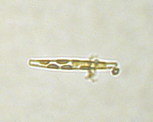
Nitzschia
Watch trend
How to distinguish
Look for the morphology expected for Nitzschia: cell outline, colony/chain pattern, pigmentation, motility if live, and whether the object matches the Diatoms functional group. Confirm difficult cases by comparing multiple micrographs and, where needed, expert taxonomy.
System effect
In the system, Nitzschia detections should be interpreted with density, trend, water colour, DO, pH and fish behaviour. A sudden increase can indicate bloom development, organic loading, or a shift in plankton community structure.
Recommended response
Repeat the slide, compare another field of view, check DO/pH, and review the Google microscopy panel before reporting species-level identity. Escalate high-risk HAB or gill-irritating classes.
Look for the morphology expected for Navicula: cell outline, colony/chain pattern, pigmentation, motility if live, and whether the object matches the Diatoms functional group. Confirm difficult cases by comparing multiple micrographs and, where needed, expert taxonomy.
System effect
In the system, Navicula detections should be interpreted with density, trend, water colour, DO, pH and fish behaviour. A sudden increase can indicate bloom development, organic loading, or a shift in plankton community structure.
Recommended response
Repeat the slide, compare another field of view, check DO/pH, and review the Google microscopy panel before reporting species-level identity. Escalate high-risk HAB or gill-irritating classes.
Look for the morphology expected for Pleurosigma: cell outline, colony/chain pattern, pigmentation, motility if live, and whether the object matches the Diatoms functional group. Confirm difficult cases by comparing multiple micrographs and, where needed, expert taxonomy.
System effect
In the system, Pleurosigma detections should be interpreted with density, trend, water colour, DO, pH and fish behaviour. A sudden increase can indicate bloom development, organic loading, or a shift in plankton community structure.
Recommended response
Repeat the slide, compare another field of view, check DO/pH, and review the Google microscopy panel before reporting species-level identity. Escalate high-risk HAB or gill-irritating classes.
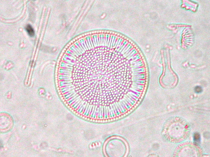
Look for the morphology expected for Cyclotella: cell outline, colony/chain pattern, pigmentation, motility if live, and whether the object matches the Diatoms functional group. Confirm difficult cases by comparing multiple micrographs and, where needed, expert taxonomy.
System effect
In the system, Cyclotella detections should be interpreted with density, trend, water colour, DO, pH and fish behaviour. A sudden increase can indicate bloom development, organic loading, or a shift in plankton community structure.
Recommended response
Repeat the slide, compare another field of view, check DO/pH, and review the Google microscopy panel before reporting species-level identity. Escalate high-risk HAB or gill-irritating classes.
Look for the morphology expected for Thalassiosira: cell outline, colony/chain pattern, pigmentation, motility if live, and whether the object matches the Diatoms functional group. Confirm difficult cases by comparing multiple micrographs and, where needed, expert taxonomy.
System effect
In the system, Thalassiosira detections should be interpreted with density, trend, water colour, DO, pH and fish behaviour. A sudden increase can indicate bloom development, organic loading, or a shift in plankton community structure.
Recommended response
Repeat the slide, compare another field of view, check DO/pH, and review the Google microscopy panel before reporting species-level identity. Escalate high-risk HAB or gill-irritating classes.
Look for the morphology expected for Chaetoceros: cell outline, colony/chain pattern, pigmentation, motility if live, and whether the object matches the Diatoms functional group. Confirm difficult cases by comparing multiple micrographs and, where needed, expert taxonomy.
System effect
In the system, Chaetoceros detections should be interpreted with density, trend, water colour, DO, pH and fish behaviour. A sudden increase can indicate bloom development, organic loading, or a shift in plankton community structure.
Recommended response
Repeat the slide, compare another field of view, check DO/pH, and review the Google microscopy panel before reporting species-level identity. Escalate high-risk HAB or gill-irritating classes.
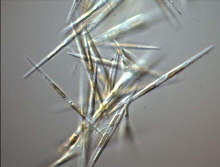
Look for the morphology expected for Pseudo-Nitzschia: cell outline, colony/chain pattern, pigmentation, motility if live, and whether the object matches the Diatoms functional group. Confirm difficult cases by comparing multiple micrographs and, where needed, expert taxonomy.
System effect
In the system, Pseudo-Nitzschia detections should be interpreted with density, trend, water colour, DO, pH and fish behaviour. A sudden increase can indicate bloom development, organic loading, or a shift in plankton community structure.
Recommended response
Repeat the slide, compare another field of view, check DO/pH, and review the Google microscopy panel before reporting species-level identity. Escalate high-risk HAB or gill-irritating classes.
Look for the morphology expected for Gyrodinium: cell outline, colony/chain pattern, pigmentation, motility if live, and whether the object matches the Dinoflagellates functional group. Confirm difficult cases by comparing multiple micrographs and, where needed, expert taxonomy.
System effect
In the system, Gyrodinium detections should be interpreted with density, trend, water colour, DO, pH and fish behaviour. A sudden increase can indicate bloom development, organic loading, or a shift in plankton community structure.
Recommended response
Repeat the slide, compare another field of view, check DO/pH, and review the Google microscopy panel before reporting species-level identity. Escalate high-risk HAB or gill-irritating classes.
Look for the morphology expected for Prorocentrum: cell outline, colony/chain pattern, pigmentation, motility if live, and whether the object matches the Dinoflagellates functional group. Confirm difficult cases by comparing multiple micrographs and, where needed, expert taxonomy.
System effect
In the system, Prorocentrum detections should be interpreted with density, trend, water colour, DO, pH and fish behaviour. A sudden increase can indicate bloom development, organic loading, or a shift in plankton community structure.
Recommended response
Repeat the slide, compare another field of view, check DO/pH, and review the Google microscopy panel before reporting species-level identity. Escalate high-risk HAB or gill-irritating classes.
Look for the morphology expected for Gymnodinium: cell outline, colony/chain pattern, pigmentation, motility if live, and whether the object matches the Dinoflagellates functional group. Confirm difficult cases by comparing multiple micrographs and, where needed, expert taxonomy.
System effect
In the system, Gymnodinium detections should be interpreted with density, trend, water colour, DO, pH and fish behaviour. A sudden increase can indicate bloom development, organic loading, or a shift in plankton community structure.
Recommended response
Repeat the slide, compare another field of view, check DO/pH, and review the Google microscopy panel before reporting species-level identity. Escalate high-risk HAB or gill-irritating classes.
Look for the morphology expected for Alexandriam: cell outline, colony/chain pattern, pigmentation, motility if live, and whether the object matches the Dinoflagellates functional group. Confirm difficult cases by comparing multiple micrographs and, where needed, expert taxonomy.
System effect
In the system, Alexandriam detections should be interpreted with density, trend, water colour, DO, pH and fish behaviour. A sudden increase can indicate bloom development, organic loading, or a shift in plankton community structure.
Recommended response
Repeat the slide, compare another field of view, check DO/pH, and review the Google microscopy panel before reporting species-level identity. Escalate high-risk HAB or gill-irritating classes.
Karlodinium microscopy reference Use the Google Images button below for current real micrographs. No unstable image URL is embedded, so this panel will not show a broken image.
How to distinguish
Look for the morphology expected for Karlodinium: cell outline, colony/chain pattern, pigmentation, motility if live, and whether the object matches the Dinoflagellates functional group. Confirm difficult cases by comparing multiple micrographs and, where needed, expert taxonomy.
System effect
In the system, Karlodinium detections should be interpreted with density, trend, water colour, DO, pH and fish behaviour. A sudden increase can indicate bloom development, organic loading, or a shift in plankton community structure.
Recommended response
Repeat the slide, compare another field of view, check DO/pH, and review the Google microscopy panel before reporting species-level identity. Escalate high-risk HAB or gill-irritating classes.
Look for the morphology expected for Ceratium: cell outline, colony/chain pattern, pigmentation, motility if live, and whether the object matches the Dinoflagellates functional group. Confirm difficult cases by comparing multiple micrographs and, where needed, expert taxonomy.
System effect
In the system, Ceratium detections should be interpreted with density, trend, water colour, DO, pH and fish behaviour. A sudden increase can indicate bloom development, organic loading, or a shift in plankton community structure.
Recommended response
Repeat the slide, compare another field of view, check DO/pH, and review the Google microscopy panel before reporting species-level identity. Escalate high-risk HAB or gill-irritating classes.
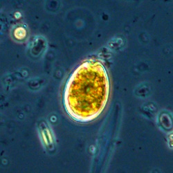
Look for the morphology expected for Chlorella: cell outline, colony/chain pattern, pigmentation, motility if live, and whether the object matches the Green Algae functional group. Confirm difficult cases by comparing multiple micrographs and, where needed, expert taxonomy.
System effect
In the system, Chlorella detections should be interpreted with density, trend, water colour, DO, pH and fish behaviour. A sudden increase can indicate bloom development, organic loading, or a shift in plankton community structure.
Recommended response
Repeat the slide, compare another field of view, check DO/pH, and review the Google microscopy panel before reporting species-level identity. Escalate high-risk HAB or gill-irritating classes.
Look for the morphology expected for Oosystis: cell outline, colony/chain pattern, pigmentation, motility if live, and whether the object matches the Green Algae functional group. Confirm difficult cases by comparing multiple micrographs and, where needed, expert taxonomy.
System effect
In the system, Oosystis detections should be interpreted with density, trend, water colour, DO, pH and fish behaviour. A sudden increase can indicate bloom development, organic loading, or a shift in plankton community structure.
Recommended response
Repeat the slide, compare another field of view, check DO/pH, and review the Google microscopy panel before reporting species-level identity. Escalate high-risk HAB or gill-irritating classes.
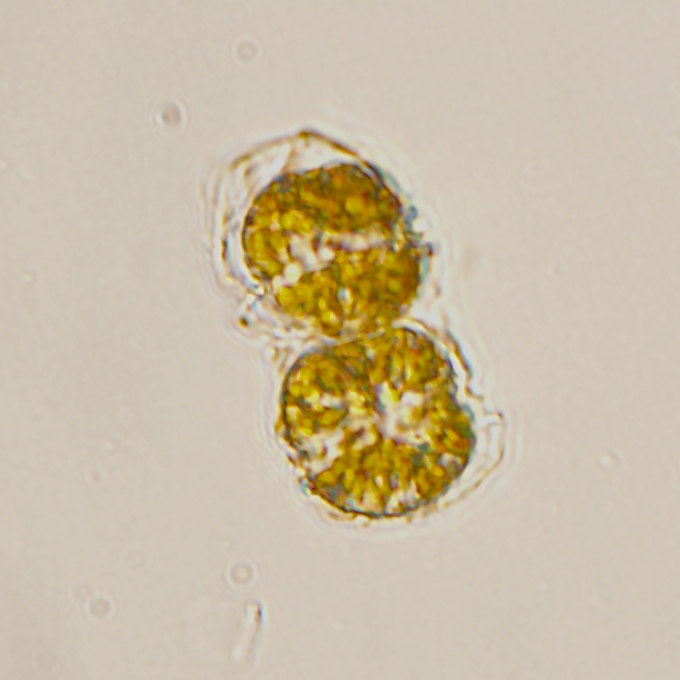
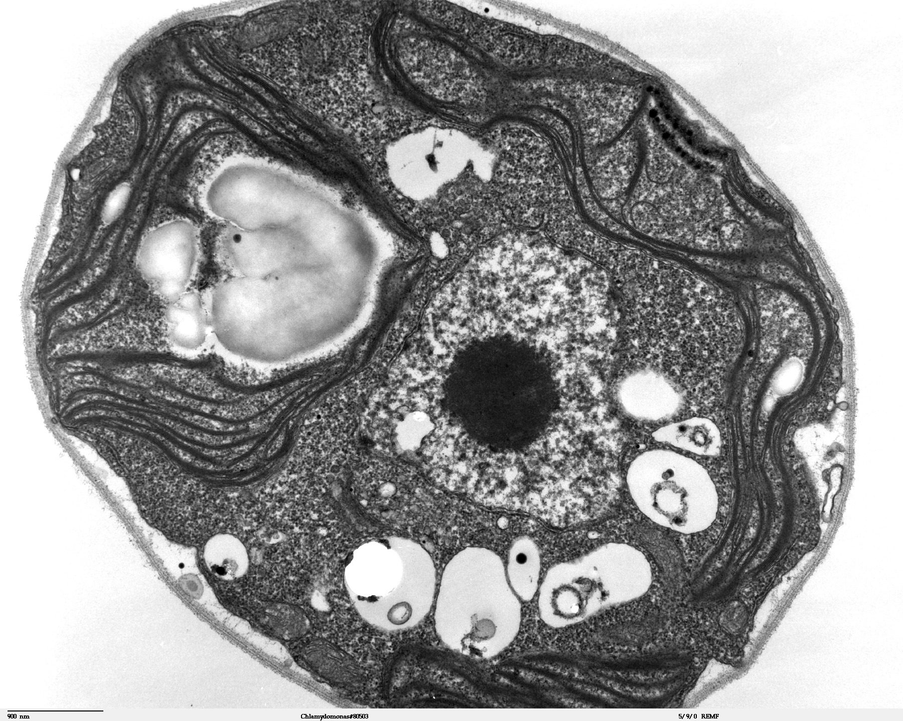
Look for the morphology expected for Chlamydomonas: cell outline, colony/chain pattern, pigmentation, motility if live, and whether the object matches the Green Algae functional group. Confirm difficult cases by comparing multiple micrographs and, where needed, expert taxonomy.
System effect
In the system, Chlamydomonas detections should be interpreted with density, trend, water colour, DO, pH and fish behaviour. A sudden increase can indicate bloom development, organic loading, or a shift in plankton community structure.
Recommended response
Repeat the slide, compare another field of view, check DO/pH, and review the Google microscopy panel before reporting species-level identity. Escalate high-risk HAB or gill-irritating classes.
Look for the morphology expected for Oocystis: cell outline, colony/chain pattern, pigmentation, motility if live, and whether the object matches the Green Algae functional group. Confirm difficult cases by comparing multiple micrographs and, where needed, expert taxonomy.
System effect
In the system, Oocystis detections should be interpreted with density, trend, water colour, DO, pH and fish behaviour. A sudden increase can indicate bloom development, organic loading, or a shift in plankton community structure.
Recommended response
Repeat the slide, compare another field of view, check DO/pH, and review the Google microscopy panel before reporting species-level identity. Escalate high-risk HAB or gill-irritating classes.
Look for the morphology expected for Anabena: cell outline, colony/chain pattern, pigmentation, motility if live, and whether the object matches the Blue green (Cyanobacteria) functional group. Confirm difficult cases by comparing multiple micrographs and, where needed, expert taxonomy.
System effect
In the system, Anabena detections should be interpreted with density, trend, water colour, DO, pH and fish behaviour. A sudden increase can indicate bloom development, organic loading, or a shift in plankton community structure.
Recommended response
Repeat the slide, compare another field of view, check DO/pH, and review the Google microscopy panel before reporting species-level identity. Escalate high-risk HAB or gill-irritating classes.
Geitlerinema microscopy reference Use the Google Images button below for current real micrographs. No unstable image URL is embedded, so this panel will not show a broken image.
How to distinguish
Look for the morphology expected for Geitlerinema: cell outline, colony/chain pattern, pigmentation, motility if live, and whether the object matches the Blue green (Cyanobacteria) functional group. Confirm difficult cases by comparing multiple micrographs and, where needed, expert taxonomy.
System effect
In the system, Geitlerinema detections should be interpreted with density, trend, water colour, DO, pH and fish behaviour. A sudden increase can indicate bloom development, organic loading, or a shift in plankton community structure.
Recommended response
Repeat the slide, compare another field of view, check DO/pH, and review the Google microscopy panel before reporting species-level identity. Escalate high-risk HAB or gill-irritating classes.
Look for the morphology expected for Chroococcus: cell outline, colony/chain pattern, pigmentation, motility if live, and whether the object matches the Blue green (Cyanobacteria) functional group. Confirm difficult cases by comparing multiple micrographs and, where needed, expert taxonomy.
System effect
In the system, Chroococcus detections should be interpreted with density, trend, water colour, DO, pH and fish behaviour. A sudden increase can indicate bloom development, organic loading, or a shift in plankton community structure.
Recommended response
Repeat the slide, compare another field of view, check DO/pH, and review the Google microscopy panel before reporting species-level identity. Escalate high-risk HAB or gill-irritating classes.
Merismopedia microscopy reference Use the Google Images button below for current real micrographs. No unstable image URL is embedded, so this panel will not show a broken image.
How to distinguish
Look for the morphology expected for Merismopedia: cell outline, colony/chain pattern, pigmentation, motility if live, and whether the object matches the Blue green (Cyanobacteria) functional group. Confirm difficult cases by comparing multiple micrographs and, where needed, expert taxonomy.
System effect
In the system, Merismopedia detections should be interpreted with density, trend, water colour, DO, pH and fish behaviour. A sudden increase can indicate bloom development, organic loading, or a shift in plankton community structure.
Recommended response
Repeat the slide, compare another field of view, check DO/pH, and review the Google microscopy panel before reporting species-level identity. Escalate high-risk HAB or gill-irritating classes.
Look for the morphology expected for Oscillatoria: cell outline, colony/chain pattern, pigmentation, motility if live, and whether the object matches the Blue green (Cyanobacteria) functional group. Confirm difficult cases by comparing multiple micrographs and, where needed, expert taxonomy.
System effect
In the system, Oscillatoria detections should be interpreted with density, trend, water colour, DO, pH and fish behaviour. A sudden increase can indicate bloom development, organic loading, or a shift in plankton community structure.
Recommended response
Repeat the slide, compare another field of view, check DO/pH, and review the Google microscopy panel before reporting species-level identity. Escalate high-risk HAB or gill-irritating classes.
Look for the morphology expected for Microcyctis: cell outline, colony/chain pattern, pigmentation, motility if live, and whether the object matches the Blue green (Cyanobacteria) functional group. Confirm difficult cases by comparing multiple micrographs and, where needed, expert taxonomy.
System effect
In the system, Microcyctis detections should be interpreted with density, trend, water colour, DO, pH and fish behaviour. A sudden increase can indicate bloom development, organic loading, or a shift in plankton community structure.
Recommended response
Repeat the slide, compare another field of view, check DO/pH, and review the Google microscopy panel before reporting species-level identity. Escalate high-risk HAB or gill-irritating classes.
Look for the morphology expected for Cyanobacteria: cell outline, colony/chain pattern, pigmentation, motility if live, and whether the object matches the Blue green (Cyanobacteria) functional group. Confirm difficult cases by comparing multiple micrographs and, where needed, expert taxonomy.
System effect
In the system, Cyanobacteria detections should be interpreted with density, trend, water colour, DO, pH and fish behaviour. A sudden increase can indicate bloom development, organic loading, or a shift in plankton community structure.
Recommended response
Repeat the slide, compare another field of view, check DO/pH, and review the Google microscopy panel before reporting species-level identity. Escalate high-risk HAB or gill-irritating classes.
Look for the morphology expected for Cynobacteria: cell outline, colony/chain pattern, pigmentation, motility if live, and whether the object matches the Blue green (Cyanobacteria) functional group. Confirm difficult cases by comparing multiple micrographs and, where needed, expert taxonomy.
System effect
In the system, Cynobacteria detections should be interpreted with density, trend, water colour, DO, pH and fish behaviour. A sudden increase can indicate bloom development, organic loading, or a shift in plankton community structure.
Recommended response
Repeat the slide, compare another field of view, check DO/pH, and review the Google microscopy panel before reporting species-level identity. Escalate high-risk HAB or gill-irritating classes.
Cryptomonds microscopy reference Use the Google Images button below for current real micrographs. No unstable image URL is embedded, so this panel will not show a broken image.
How to distinguish
Look for the morphology expected for Cryptomonds: cell outline, colony/chain pattern, pigmentation, motility if live, and whether the object matches the Cryptomonds functional group. Confirm difficult cases by comparing multiple micrographs and, where needed, expert taxonomy.
System effect
In the system, Cryptomonds detections should be interpreted with density, trend, water colour, DO, pH and fish behaviour. A sudden increase can indicate bloom development, organic loading, or a shift in plankton community structure.
Recommended response
Repeat the slide, compare another field of view, check DO/pH, and review the Google microscopy panel before reporting species-level identity. Escalate high-risk HAB or gill-irritating classes.
Picoplankton microscopy reference Use the Google Images button below for current real micrographs. No unstable image URL is embedded, so this panel will not show a broken image.
How to distinguish
Look for the morphology expected for Picoplankton: cell outline, colony/chain pattern, pigmentation, motility if live, and whether the object matches the Eustigmatophytes functional group. Confirm difficult cases by comparing multiple micrographs and, where needed, expert taxonomy.
System effect
In the system, Picoplankton detections should be interpreted with density, trend, water colour, DO, pH and fish behaviour. A sudden increase can indicate bloom development, organic loading, or a shift in plankton community structure.
Recommended response
Repeat the slide, compare another field of view, check DO/pH, and review the Google microscopy panel before reporting species-level identity. Escalate high-risk HAB or gill-irritating classes.
Heliozoans microscopy reference Use the Google Images button below for current real micrographs. No unstable image URL is embedded, so this panel will not show a broken image.
How to distinguish
Look for the morphology expected for Heliozoans: cell outline, colony/chain pattern, pigmentation, motility if live, and whether the object matches the Heliozoa functional group. Confirm difficult cases by comparing multiple micrographs and, where needed, expert taxonomy.
System effect
In the system, Heliozoans detections should be interpreted with density, trend, water colour, DO, pH and fish behaviour. A sudden increase can indicate bloom development, organic loading, or a shift in plankton community structure.
Recommended response
Repeat the slide, compare another field of view, check DO/pH, and review the Google microscopy panel before reporting species-level identity. Escalate high-risk HAB or gill-irritating classes.
Euglenoid microscopy reference Use the Google Images button below for current real micrographs. No unstable image URL is embedded, so this panel will not show a broken image.
How to distinguish
Look for the morphology expected for Euglenoid: cell outline, colony/chain pattern, pigmentation, motility if live, and whether the object matches the Euglena functional group. Confirm difficult cases by comparing multiple micrographs and, where needed, expert taxonomy.
System effect
In the system, Euglenoid detections should be interpreted with density, trend, water colour, DO, pH and fish behaviour. A sudden increase can indicate bloom development, organic loading, or a shift in plankton community structure.
Recommended response
Repeat the slide, compare another field of view, check DO/pH, and review the Google microscopy panel before reporting species-level identity. Escalate high-risk HAB or gill-irritating classes.
Euglenoid Eutreptiella microscopy reference Use the Google Images button below for current real micrographs. No unstable image URL is embedded, so this panel will not show a broken image.
How to distinguish
Look for the morphology expected for Euglenoid Eutreptiella: cell outline, colony/chain pattern, pigmentation, motility if live, and whether the object matches the Euglena functional group. Confirm difficult cases by comparing multiple micrographs and, where needed, expert taxonomy.
System effect
In the system, Euglenoid Eutreptiella detections should be interpreted with density, trend, water colour, DO, pH and fish behaviour. A sudden increase can indicate bloom development, organic loading, or a shift in plankton community structure.
Recommended response
Repeat the slide, compare another field of view, check DO/pH, and review the Google microscopy panel before reporting species-level identity. Escalate high-risk HAB or gill-irritating classes.
Look for the morphology expected for Prymnesium: cell outline, colony/chain pattern, pigmentation, motility if live, and whether the object matches the Haptophyte functional group. Confirm difficult cases by comparing multiple micrographs and, where needed, expert taxonomy.
System effect
In the system, Prymnesium detections should be interpreted with density, trend, water colour, DO, pH and fish behaviour. A sudden increase can indicate bloom development, organic loading, or a shift in plankton community structure.
Recommended response
Repeat the slide, compare another field of view, check DO/pH, and review the Google microscopy panel before reporting species-level identity. Escalate high-risk HAB or gill-irritating classes.
Look for the morphology expected for Heterosigma: cell outline, colony/chain pattern, pigmentation, motility if live, and whether the object matches the Raphidophyte functional group. Confirm difficult cases by comparing multiple micrographs and, where needed, expert taxonomy.
System effect
In the system, Heterosigma detections should be interpreted with density, trend, water colour, DO, pH and fish behaviour. A sudden increase can indicate bloom development, organic loading, or a shift in plankton community structure.
Recommended response
Repeat the slide, compare another field of view, check DO/pH, and review the Google microscopy panel before reporting species-level identity. Escalate high-risk HAB or gill-irritating classes.
Chattonella microscopy reference Use the Google Images button below for current real micrographs. No unstable image URL is embedded, so this panel will not show a broken image.
How to distinguish
Look for the morphology expected for Chattonella: cell outline, colony/chain pattern, pigmentation, motility if live, and whether the object matches the Raphidophyte functional group. Confirm difficult cases by comparing multiple micrographs and, where needed, expert taxonomy.
System effect
In the system, Chattonella detections should be interpreted with density, trend, water colour, DO, pH and fish behaviour. A sudden increase can indicate bloom development, organic loading, or a shift in plankton community structure.
Recommended response
Repeat the slide, compare another field of view, check DO/pH, and review the Google microscopy panel before reporting species-level identity. Escalate high-risk HAB or gill-irritating classes.
macro-algae microscopy reference Use the Google Images button below for current real micrographs. No unstable image URL is embedded, so this panel will not show a broken image.
How to distinguish
Look for the morphology expected for macro-algae: cell outline, colony/chain pattern, pigmentation, motility if live, and whether the object matches the Macro Algae functional group. Confirm difficult cases by comparing multiple micrographs and, where needed, expert taxonomy.
System effect
In the system, macro-algae detections should be interpreted with density, trend, water colour, DO, pH and fish behaviour. A sudden increase can indicate bloom development, organic loading, or a shift in plankton community structure.
Recommended response
Repeat the slide, compare another field of view, check DO/pH, and review the Google microscopy panel before reporting species-level identity. Escalate high-risk HAB or gill-irritating classes.
New microscopy reference Use the Google Images button below for current real micrographs. No unstable image URL is embedded, so this panel will not show a broken image.
How to distinguish
Look for the morphology expected for New: cell outline, colony/chain pattern, pigmentation, motility if live, and whether the object matches the Other functional group. Confirm difficult cases by comparing multiple micrographs and, where needed, expert taxonomy.
System effect
In the system, New detections should be interpreted with density, trend, water colour, DO, pH and fish behaviour. A sudden increase can indicate bloom development, organic loading, or a shift in plankton community structure.
Recommended response
Repeat the slide, compare another field of view, check DO/pH, and review the Google microscopy panel before reporting species-level identity. Escalate high-risk HAB or gill-irritating classes.
Identify Red blood cells / erythrocytes by cell size, nuclear shape, cytoplasmic colour/granules, thrombocyte/RBC background, and smear quality. Fish blood cells can differ from mammalian examples, so treat this as morphology guidance.
System effect
Changes in Red blood cells / erythrocytes proportions can suggest stress, inflammation, immune activation, handling effects, or smear artefact. Interpretation must be linked to fish condition and water quality.
Recommended response
Review smear quality, staining, duplicate fields, and if abnormal patterns persist, confirm with fish-health/veterinary review.
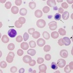
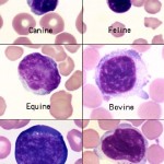
Identify Lymphocytes by cell size, nuclear shape, cytoplasmic colour/granules, thrombocyte/RBC background, and smear quality. Fish blood cells can differ from mammalian examples, so treat this as morphology guidance.
System effect
Changes in Lymphocytes proportions can suggest stress, inflammation, immune activation, handling effects, or smear artefact. Interpretation must be linked to fish condition and water quality.
Recommended response
Review smear quality, staining, duplicate fields, and if abnormal patterns persist, confirm with fish-health/veterinary review.
Identify Thrombocytes by cell size, nuclear shape, cytoplasmic colour/granules, thrombocyte/RBC background, and smear quality. Fish blood cells can differ from mammalian examples, so treat this as morphology guidance.
System effect
Changes in Thrombocytes proportions can suggest stress, inflammation, immune activation, handling effects, or smear artefact. Interpretation must be linked to fish condition and water quality.
Recommended response
Review smear quality, staining, duplicate fields, and if abnormal patterns persist, confirm with fish-health/veterinary review.
Identify Monocytes by cell size, nuclear shape, cytoplasmic colour/granules, thrombocyte/RBC background, and smear quality. Fish blood cells can differ from mammalian examples, so treat this as morphology guidance.
System effect
Changes in Monocytes proportions can suggest stress, inflammation, immune activation, handling effects, or smear artefact. Interpretation must be linked to fish condition and water quality.
Recommended response
Review smear quality, staining, duplicate fields, and if abnormal patterns persist, confirm with fish-health/veterinary review.
Identify Neutrophil / heterophil-like granulocytes by cell size, nuclear shape, cytoplasmic colour/granules, thrombocyte/RBC background, and smear quality. Fish blood cells can differ from mammalian examples, so treat this as morphology guidance.
System effect
Changes in Neutrophil / heterophil-like granulocytes proportions can suggest stress, inflammation, immune activation, handling effects, or smear artefact. Interpretation must be linked to fish condition and water quality.
Recommended response
Review smear quality, staining, duplicate fields, and if abnormal patterns persist, confirm with fish-health/veterinary review.
Identify Eosinophil-like granulocytes by cell size, nuclear shape, cytoplasmic colour/granules, thrombocyte/RBC background, and smear quality. Fish blood cells can differ from mammalian examples, so treat this as morphology guidance.
System effect
Changes in Eosinophil-like granulocytes proportions can suggest stress, inflammation, immune activation, handling effects, or smear artefact. Interpretation must be linked to fish condition and water quality.
Recommended response
Review smear quality, staining, duplicate fields, and if abnormal patterns persist, confirm with fish-health/veterinary review.
Identify Basophil-like granulocytes by cell size, nuclear shape, cytoplasmic colour/granules, thrombocyte/RBC background, and smear quality. Fish blood cells can differ from mammalian examples, so treat this as morphology guidance.
System effect
Changes in Basophil-like granulocytes proportions can suggest stress, inflammation, immune activation, handling effects, or smear artefact. Interpretation must be linked to fish condition and water quality.
Recommended response
Review smear quality, staining, duplicate fields, and if abnormal patterns persist, confirm with fish-health/veterinary review.
Artefact / immature-cell review microscopy reference Use the Google Images button below for current real micrographs. No unstable image URL is embedded, so this panel will not show a broken image.
How to distinguish
Identify Artefact / immature-cell review by cell size, nuclear shape, cytoplasmic colour/granules, thrombocyte/RBC background, and smear quality. Fish blood cells can differ from mammalian examples, so treat this as morphology guidance.
System effect
Changes in Artefact / immature-cell review proportions can suggest stress, inflammation, immune activation, handling effects, or smear artefact. Interpretation must be linked to fish condition and water quality.
Recommended response
Review smear quality, staining, duplicate fields, and if abnormal patterns persist, confirm with fish-health/veterinary review.
Gill Trichodina microscopy reference Use the Google Images button below for current real micrographs. No unstable image URL is embedded, so this panel will not show a broken image.
How to distinguish
Gill Trichodina is reviewed as a gill/skin health-screening label. Look for the organism or lesion pattern in the correct tissue context, not as a free-floating water-column label.
System effect
A positive Gill Trichodina trend may indicate parasite burden, bacterial irritation, epithelial damage, mucus response, or secondary infection pressure. Interpret with wet mount quality and clinical signs.
Recommended response
Repeat wet mount, check fish behaviour, gill colour and mucus, record affected site, and confirm with laboratory/veterinary review when counts or clinical signs increase.
Gill Amyloodinium microscopy reference Use the Google Images button below for current real micrographs. No unstable image URL is embedded, so this panel will not show a broken image.
How to distinguish
Gill Amyloodinium is reviewed as a gill/skin health-screening label. Look for the organism or lesion pattern in the correct tissue context, not as a free-floating water-column label.
System effect
A positive Gill Amyloodinium trend may indicate parasite burden, bacterial irritation, epithelial damage, mucus response, or secondary infection pressure. Interpret with wet mount quality and clinical signs.
Recommended response
Repeat wet mount, check fish behaviour, gill colour and mucus, record affected site, and confirm with laboratory/veterinary review when counts or clinical signs increase.
Gill Bacterial infection microscopy reference Use the Google Images button below for current real micrographs. No unstable image URL is embedded, so this panel will not show a broken image.
How to distinguish
Gill Bacterial infection is reviewed as a gill/skin health-screening label. Look for the organism or lesion pattern in the correct tissue context, not as a free-floating water-column label.
System effect
A positive Gill Bacterial infection trend may indicate parasite burden, bacterial irritation, epithelial damage, mucus response, or secondary infection pressure. Interpret with wet mount quality and clinical signs.
Recommended response
Repeat wet mount, check fish behaviour, gill colour and mucus, record affected site, and confirm with laboratory/veterinary review when counts or clinical signs increase.
Gill Amoeba microscopy reference Use the Google Images button below for current real micrographs. No unstable image URL is embedded, so this panel will not show a broken image.
How to distinguish
Gill Amoeba is reviewed as a gill/skin health-screening label. Look for the organism or lesion pattern in the correct tissue context, not as a free-floating water-column label.
System effect
A positive Gill Amoeba trend may indicate parasite burden, bacterial irritation, epithelial damage, mucus response, or secondary infection pressure. Interpret with wet mount quality and clinical signs.
Recommended response
Repeat wet mount, check fish behaviour, gill colour and mucus, record affected site, and confirm with laboratory/veterinary review when counts or clinical signs increase.
Gill Fluke microscopy reference Use the Google Images button below for current real micrographs. No unstable image URL is embedded, so this panel will not show a broken image.
How to distinguish
Gill Fluke is reviewed as a gill/skin health-screening label. Look for the organism or lesion pattern in the correct tissue context, not as a free-floating water-column label.
System effect
A positive Gill Fluke trend may indicate parasite burden, bacterial irritation, epithelial damage, mucus response, or secondary infection pressure. Interpret with wet mount quality and clinical signs.
Recommended response
Repeat wet mount, check fish behaviour, gill colour and mucus, record affected site, and confirm with laboratory/veterinary review when counts or clinical signs increase.
Skin Saprolegnia microscopy reference Use the Google Images button below for current real micrographs. No unstable image URL is embedded, so this panel will not show a broken image.
How to distinguish
Skin Saprolegnia is reviewed as a gill/skin health-screening label. Look for the organism or lesion pattern in the correct tissue context, not as a free-floating water-column label.
System effect
A positive Skin Saprolegnia trend may indicate parasite burden, bacterial irritation, epithelial damage, mucus response, or secondary infection pressure. Interpret with wet mount quality and clinical signs.
Recommended response
Repeat wet mount, check fish behaviour, gill colour and mucus, record affected site, and confirm with laboratory/veterinary review when counts or clinical signs increase.
Skin Trichodina microscopy reference Use the Google Images button below for current real micrographs. No unstable image URL is embedded, so this panel will not show a broken image.
How to distinguish
Skin Trichodina is reviewed as a gill/skin health-screening label. Look for the organism or lesion pattern in the correct tissue context, not as a free-floating water-column label.
System effect
A positive Skin Trichodina trend may indicate parasite burden, bacterial irritation, epithelial damage, mucus response, or secondary infection pressure. Interpret with wet mount quality and clinical signs.
Recommended response
Repeat wet mount, check fish behaviour, gill colour and mucus, record affected site, and confirm with laboratory/veterinary review when counts or clinical signs increase.
Skin Bacterial infection microscopy reference Use the Google Images button below for current real micrographs. No unstable image URL is embedded, so this panel will not show a broken image.
How to distinguish
Skin Bacterial infection is reviewed as a gill/skin health-screening label. Look for the organism or lesion pattern in the correct tissue context, not as a free-floating water-column label.
System effect
A positive Skin Bacterial infection trend may indicate parasite burden, bacterial irritation, epithelial damage, mucus response, or secondary infection pressure. Interpret with wet mount quality and clinical signs.
Recommended response
Repeat wet mount, check fish behaviour, gill colour and mucus, record affected site, and confirm with laboratory/veterinary review when counts or clinical signs increase.
Skin Ich microscopy reference Use the Google Images button below for current real micrographs. No unstable image URL is embedded, so this panel will not show a broken image.
How to distinguish
Skin Ich is reviewed as a gill/skin health-screening label. Look for the organism or lesion pattern in the correct tissue context, not as a free-floating water-column label.
System effect
A positive Skin Ich trend may indicate parasite burden, bacterial irritation, epithelial damage, mucus response, or secondary infection pressure. Interpret with wet mount quality and clinical signs.
Recommended response
Repeat wet mount, check fish behaviour, gill colour and mucus, record affected site, and confirm with laboratory/veterinary review when counts or clinical signs increase.
Skin Costia microscopy reference Use the Google Images button below for current real micrographs. No unstable image URL is embedded, so this panel will not show a broken image.
How to distinguish
Skin Costia is reviewed as a gill/skin health-screening label. Look for the organism or lesion pattern in the correct tissue context, not as a free-floating water-column label.
System effect
A positive Skin Costia trend may indicate parasite burden, bacterial irritation, epithelial damage, mucus response, or secondary infection pressure. Interpret with wet mount quality and clinical signs.
Recommended response
Repeat wet mount, check fish behaviour, gill colour and mucus, record affected site, and confirm with laboratory/veterinary review when counts or clinical signs increase.
Skin Fluke microscopy reference Use the Google Images button below for current real micrographs. No unstable image URL is embedded, so this panel will not show a broken image.
How to distinguish
Skin Fluke is reviewed as a gill/skin health-screening label. Look for the organism or lesion pattern in the correct tissue context, not as a free-floating water-column label.
System effect
A positive Skin Fluke trend may indicate parasite burden, bacterial irritation, epithelial damage, mucus response, or secondary infection pressure. Interpret with wet mount quality and clinical signs.
Recommended response
Repeat wet mount, check fish behaviour, gill colour and mucus, record affected site, and confirm with laboratory/veterinary review when counts or clinical signs increase.
Rotifiers microscopy reference Use the Google Images button below for current real micrographs. No unstable image URL is embedded, so this panel will not show a broken image.
How to distinguish
Rotifiers is a live-feed/egg/cyst class. Confirm by size, swimming behaviour, body segmentation or cyst shell, and by whether the sample came from live-feed culture rather than fish tissue.
System effect
Rotifiers abundance informs feed availability, hatchery culture status, contamination, or background plankton entering the sample.
Recommended response
Use counts for culture monitoring and quality checks; repeat if debris, bubbles, or mixed cultures create false detections.
Artemia microscopy reference Use the Google Images button below for current real micrographs. No unstable image URL is embedded, so this panel will not show a broken image.
How to distinguish
Artemia is a live-feed/egg/cyst class. Confirm by size, swimming behaviour, body segmentation or cyst shell, and by whether the sample came from live-feed culture rather than fish tissue.
System effect
Artemia abundance informs feed availability, hatchery culture status, contamination, or background plankton entering the sample.
Recommended response
Use counts for culture monitoring and quality checks; repeat if debris, bubbles, or mixed cultures create false detections.
Copepods microscopy reference Use the Google Images button below for current real micrographs. No unstable image URL is embedded, so this panel will not show a broken image.
How to distinguish
Copepods is a live-feed/egg/cyst class. Confirm by size, swimming behaviour, body segmentation or cyst shell, and by whether the sample came from live-feed culture rather than fish tissue.
System effect
Copepods abundance informs feed availability, hatchery culture status, contamination, or background plankton entering the sample.
Recommended response
Use counts for culture monitoring and quality checks; repeat if debris, bubbles, or mixed cultures create false detections.
Rotifiers Eggs microscopy reference Use the Google Images button below for current real micrographs. No unstable image URL is embedded, so this panel will not show a broken image.
How to distinguish
Rotifiers Eggs is a live-feed/egg/cyst class. Confirm by size, swimming behaviour, body segmentation or cyst shell, and by whether the sample came from live-feed culture rather than fish tissue.
System effect
Rotifiers Eggs abundance informs feed availability, hatchery culture status, contamination, or background plankton entering the sample.
Recommended response
Use counts for culture monitoring and quality checks; repeat if debris, bubbles, or mixed cultures create false detections.
Artemia Cysts microscopy reference Use the Google Images button below for current real micrographs. No unstable image URL is embedded, so this panel will not show a broken image.
How to distinguish
Artemia Cysts is a live-feed/egg/cyst class. Confirm by size, swimming behaviour, body segmentation or cyst shell, and by whether the sample came from live-feed culture rather than fish tissue.
System effect
Artemia Cysts abundance informs feed availability, hatchery culture status, contamination, or background plankton entering the sample.
Recommended response
Use counts for culture monitoring and quality checks; repeat if debris, bubbles, or mixed cultures create false detections.
Eggs microscopy reference Use the Google Images button below for current real micrographs. No unstable image URL is embedded, so this panel will not show a broken image.
How to distinguish
Eggs is a live-feed/egg/cyst class. Confirm by size, swimming behaviour, body segmentation or cyst shell, and by whether the sample came from live-feed culture rather than fish tissue.
System effect
Eggs abundance informs feed availability, hatchery culture status, contamination, or background plankton entering the sample.
Recommended response
Use counts for culture monitoring and quality checks; repeat if debris, bubbles, or mixed cultures create false detections.
Use this section when installing DPKAI Aqualab v0.1 on a new Windows computer. The recommended installation path is now the project repository, so the full folder can be cloned, updated, and maintained consistently. The main application file name should be dpkai_aqualab_v0.1.py.
1. Recommended method: clone the project folder from GitHub
Install Git for Windows first, then open Command Prompt or PowerShell in the parent folder where the project should live, for example the Desktop.
cd %USERPROFILE%\Desktop
git clone https://github.com/dpkpandey/aqaulab.git
cd aqaulab
This creates a clean working directory containing the application files. If the repository is private, log in to GitHub or use the correct access token/credential when prompted.
If the system is installed from a USB drive, ZIP file, or shared folder, create one folder and copy the complete application package into it:
C:\Users\YourName\Desktop\DPKAI_Aqualab\
Do not run the program from Downloads, a temporary ZIP preview, or a random terminal directory. The working directory must contain the script, support files, model files, licence files, logos, and output folders together.
3. Required files in the working directory
dpkai_aqualab_v0.1.py — main application script
editable_measure.py — calibration, ROI and length drawing support
requirements.txt — Python package list for repeatable installation
logo/ — DPKAI Aqualab and Barra Vision icons
License/ — licence and terms files
algae.pt, wbc.pt, bacteria.pt, total_algae.pt, live_feed.pt or the active model files used by the deployment
Keep file names consistent. If a model file is renamed, update the application setting or file selection accordingly before routine use.
4. Install Python
Install Python 3.10 or 3.11 from the official Python installer. During installation, select Add Python to PATH. After installation, open Command Prompt and confirm:
python --version
pip --version
If Windows does not recognise python, close and reopen the terminal, or use py instead of python.
5. Create and activate a virtual environment
Run these commands inside the cloned or copied project folder:
cd %USERPROFILE%\Desktop\aqaulab
python -m venv myenv
myenv\Scripts\activate
The terminal should show (myenv). Install and run the software only while this environment is active.
6. Install required modules from requirements.txt
The clean professional method is to install from the project requirement file:
For GPU-enabled deployments, install the correct Torch build for the installed CUDA driver. Confirm GPU availability only after the software opens correctly in CPU mode.
7. Confirm the working directory layout
The application creates and uses local folders beside the script:
images/ — saved annotated images
Detected Footage/ — saved annotated videos
Dashboard images/ — exported graphs
data/ — SQLite databases and UI settings
2026_ExcelDatabase.xlsx or the current yearly Excel export
Keep these folders inside the application directory so database, image, video, and Excel records stay linked.
8. First launch
python dpkai_aqualab_v0.1.py
Confirm that the window opens, the DPKAI Aqualab / Barra Vision branding appears, the Site Information fields are visible, and the first detection mode loads correctly. Do not start routine analysis until the first launch is verified.
9. Camera and image validation
Use Cam # and Test before starting a live microscope/camera feed.
Test one still image first to confirm detection display.
Then test one short video to confirm stable playback and saving.
Run one detection and confirm that database records, Excel export, and saved image/footage folders update correctly.
10. Updating from GitHub
When the project is installed by Git clone, update it from inside the project folder:
cd %USERPROFILE%\Desktop\aqaulab
git pull
myenv\Scripts\activate
pip install -r requirements.txt
Before updating, back up the data/ folder, Excel files, saved images, saved footage, and model files. Do not overwrite operational records without a backup.
11. Deployment checklist
Keep the working directory unchanged after installation.
Back up data/, Excel files, saved images, saved footage, and model files weekly.
Do not rename model files unless the matching application setting is updated.
For Cloudflare manual hosting, upload this HTML manual as a static page only. Do not upload local databases, model files, private licence files, or operational data.
Keep the GitHub repository link in this installation section so future computers can be installed consistently using git clone.